A short survey of Bayesian Neural Networks

This concise overview introduces Bayesian Neural Networks (BNNs) as a promising alternative to standard neural networks (SNNs), which often suffer from a lack of interpretability, earning them the label of "black box" models. This lack of transparency is especially critical in the sciences and medicine, where point estimates are not sufficient and uncertainty estimates are often required. Furthermore, it is argued that incorporating Bayesian concepts into machine learning can also improve the overall accuracy of models. After an introduction and comparison between BNNs and SNNs we introduce the current understanding of a model's ability to generalize and current shortcomings, such as double descent that plagues standard neural networks, and how certain BNN frameworks prove to be a promising candidate in alleviating some of those pitfalls. However, BNNs still suffer in practical implementations due to their inferior scalability to larger datasets and models. Some of the most common approximations to the optimization of training and estimation of Bayesian statistical quantities are then introduced. To conclude this review we briefly summarize an application of uncertainty estimation with BNNs applied to cosmology.

Bayesian Neural Networks

Modern deep-learning methods are incredibly powerful tools that can tackle a wide range of challenging problems. However, due to their nature as black boxes, quantifying the uncertainty associated with their predictions can be difficult.^[1] Bayesian statistics provide a formal framework to comprehend and measure the uncertainty inherent in deep neural network predictions.

Bayesian Neural Networks incorporate the principles of Bayesian inference, which can be particularly useful when dealing with limited data or when making predictions in uncertain environments. BNNs extend traditional neural networks by introducing probabilistic weights and biases.

BNNs train the model weights as probability distributions rather than searching for a singular optimal value as with SNNs. This makes them more robust and allows them to generalize better with less overfitting. The process of finding these distributions associated with the weights is called marginalization.

A standard neural network finds point estimates of its weights through Maximum Likelihood Estimation (MLE), whereas a BNN instead reports a Maximum A Posteriori (MAP) estimate or the full predictive distribution. Where an SNN locates its optimal value by differentiation and gradient descent, a BNN relies on Markov Chain Monte Carlo (MCMC), Variational Inference, and Normalizing Flows,^[2] since the Bayesian setup involves hard-to-compute integrals. The unfortunate consequence is a marked increase in computational complexity.

Advantages of BNNs

Sources of uncertainty

Usually, in SNN applications, our data $\mathcal{D}$ is merely a sample of the process we are modeling. In these cases, we are looking for models that generalize to unseen data. Therefore, it is useful to express the uncertainty about our model due to the lack of data. This uncertainty is commonly referred to as epistemic uncertainty or parameter uncertainty.

BNNs address epistemic uncertainty, as explained above, by treating the model's weights as probabilistic variables rather than fixed parameters. This allows the model to capture the uncertainty in its own parameters and produce probabilistic predictions, indicating the model's confidence in its predictions.

There is usually a second source of uncertainty, called aleatoric uncertainty, which originates directly from the process we are modeling. This uncertainty, also known as data uncertainty, arises from the inherent variability in the data itself, the noise in the labels that cannot be explained by the inputs. It is often called "irreducible noise". Bayesian Neural Networks also help quantify and manage aleatoric uncertainty, by carrying uncertainty estimates through to the model's output.

Bayesian Inference

In Bayesian inference, given for example some known input-output pairs in a supervised learning setting, we seek to compute the posterior $p(\boldsymbol{\theta}|\mathcal{D})$ , which is the conditional distribution of the parameters of a model given the training data $\mathcal{D}$ . The posterior can be determined using Bayes' theorem:

p(\boldsymbol{\theta} | \mathcal{D})=\frac{p(\boldsymbol{\theta}) p(\mathcal{D} | \boldsymbol{\theta})}{p(\mathcal{D})} \propto p(\boldsymbol{\theta}) p(\mathcal{D}|\boldsymbol{\theta}),

where $p(\mathcal{D}|\boldsymbol{\theta})$ represents the likelihood and $p(\boldsymbol{\theta})$ the prior. Our interest in the posterior $p(\boldsymbol{\theta}|\mathcal{D})$ lies in the fact that we want to compute the posterior predictive distribution to model unseen data,

p(\boldsymbol{y}|\boldsymbol{x},\mathcal{D}) = \int p(\boldsymbol{y}|\boldsymbol{x}, \boldsymbol{\theta} ) p(\boldsymbol{\theta}|\mathcal{D})\,d\boldsymbol{\theta}= \mathbb{E}_{p(\boldsymbol{\theta}|\mathcal{D})}\left[ p(\boldsymbol{y}|\boldsymbol{x},\mathcal{D}) \right].

Equation (2) represents a Bayesian Model Average (BMA) as it averages the predictions of all plausible models weighted by their posterior. This yields a nice interpretation of the predictive distribution as an infinite ensemble of networks, hence ensemble learning, which can represent many hypothesis models we believe to be possible. This is in net contrast to MLE methods in SNNs where only one set of parameters $\boldsymbol{\theta}^*$ , therefore one hypothesized model, is used for predictions.

SNN		BNN
$\boldsymbol{\theta}^*$	$\Rightarrow$	$p(\boldsymbol{\theta}\mid\mathcal{D})$
$y_{\boldsymbol{\theta}^*}(x)$	$\Rightarrow$	$p(\boldsymbol{y}_{\boldsymbol{\theta}}\mid\boldsymbol{x},\mathcal{D})$

An immediate benefit of placing distributions over the model parameters and predictions is that we can quantify our uncertainty about them, for instance by computing their variance. This is especially relevant when learning from small datasets; standard neural net training will overfit for the reasons discussed above, but Bayesian inference will find the best explanation for the model parameters given the available data, which typically has high uncertainty when data is scarce. In the limit of dataset size far exceeding the number of neurons, the inferred distributions sharpen and begin to resemble the solutions from standard training; for modern networks we don't typically reach this limit in practice, so having a notion of model uncertainty is helpful.

The classical training of an SNN can be viewed as a limit of Bayesian inference in the case when $p(\boldsymbol{\theta}|\mathcal{D})\approx \delta(\boldsymbol{\theta}=\boldsymbol{\theta}^*)$ , where the delta function is zero everywhere except at $\boldsymbol{\theta}^*=\text{argmax}_{\boldsymbol{\theta}}\,p(\boldsymbol{\theta}|\mathcal{D})$ . The difference between a classical and Bayesian approach will depend on how sharp the posterior becomes. If the posterior is sharply peaked and the predictive distribution does not vary much where the posterior has mass, then there may be no difference between the two approaches. However, in modern SNN problems the likelihood $p(\mathcal{D}|\boldsymbol{\theta})$ has wide support, not favoring a specific set of parameters. In such scenarios, it is advantageous to employ BNNs.

In Bayesian machine learning, the prior $p(\boldsymbol{\theta})$ is often imposed. Common choices include a pre-determined class, such as Gaussian priors $p(\boldsymbol{\theta}) = \mathcal{N}(\alpha, \beta)$ , or a more systematic approach trying to estimate the parameters of the prior from the data with the help of an empirical Bayes approach.

Two computationally difficult integrals arise during the Bayesian setup which limit its use in practical applications. The first one arises from the computation of the marginal likelihood $p(\mathcal{D})=\int p(\mathcal{D} | \boldsymbol{\theta}) p(\boldsymbol{\theta})\, d \boldsymbol{\theta}$ , while the second corresponds to the posterior predictive distribution (2). It is possible to estimate these two integrals via various algorithms which can be categorized as either sampling-based or variational.

Sampling algorithms are mostly based on Markov Chain Monte Carlo (MCMC) methods; the most relevant in BNNs is the Metropolis-Hastings algorithm. For example, we can compute $p(y|x,\mathcal{D})$ by sampling a finite set of parameters $\{\theta_1, \theta_2, \ldots, \theta_N \}$ , whose distribution matches $p(\boldsymbol{\theta} | \mathcal{D})$ in the limit of large $N$ , to compute the predictive distribution. When the size of the model grows, however, sampling algorithms become less efficient, and variational algorithms are preferred when computing intractable distributions like the posterior.

Variational methods directly model the posterior using a parametrized distribution $q_{\boldsymbol{\phi}}(\boldsymbol{\theta})$ , then iteratively improve the approximation via an optimization problem. The measure of closeness that is commonly used is the Kullback-Leibler divergence shown in equation (24).^[3] The process of learning the parameters of the distribution closely resembles SNN training and is called stochastic variational inference.

Generalization

Typically, in traditional machine learning, a model's ability to generalize effectively (low generalization error) is linked to a small difference between training and test errors. However, a seminal paper by Zhang et al.^[4] revealed that even large neural networks with very small training and test errors can fit random labels in the training data, highlighting a lack of understanding in quantifying a model's generalization capacity. Moreover, in the following section, we will discuss a peculiar phenomenon known as Double Descent,^[5] which further accentuates this observation.

In the paper by Wilson et al.^[6] it is argued that the random labeling is not surprising if analyzed through a Bayesian framework with the help of the concepts of support and inductive bias. Inductive bias refers to the inherent assumptions or preferences a machine learning model acquires from its training data, guiding it to favor particular solutions over others and enabling it to generalize well to new data. This bias plays a crucial role in helping the model make sensible decisions even in the presence of noisy or limited training data. A good inductive bias is commonly encouraged through techniques such as regularization, dropout, early stopping, and data augmentation. Just as important is choosing a model architecture that strikes a balance between complexity and representational capacity.

Models with fewer parameters tend to possess a stronger inductive bias, primarily because they are constrained to fit a specific class of data. However, this limitation may also result in insufficient generalization to other types of data, as the model's support might not be extensive enough. In this context, support refers to the range of dataset classes that a model can effectively accommodate, corresponding to situations where the likelihood $p(\mathcal{D}|\mathcal{M}) > 0$ .

Thus, from a statistical perspective, we want a large support and specific inductive bias of a model to generalize well, as will become evident in the next subsection.

Marginal likelihood versus datasets for different model classes — Figure 1. The vertical axis represents the marginal likelihood or Bayesian evidence and represents how good a model is at fitting a specific dataset. Figure taken from reference [6].

Prior hypothesis space and posterior for CNN, linear model and MLP — Figure 2. Prior hypothesis space and posterior for (b) CNN, (c) linear model, (d) MLP.

Generalization for BNNs

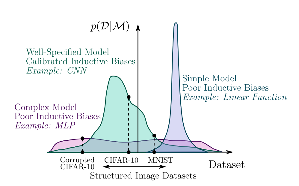
To exemplify the delicate balance between a wide support and a strong inductive bias, consider the illustration presented in Figure 1 from Wilson et al.^[6] The blue linear model displays truncated support, as it lacks the flexibility to capture quadratic behaviors in the data. Consequently, the marginal likelihood's probability mass is sharply concentrated around datasets with linear behaviors.

In contrast, a traditional MLP (multi-layer perceptron) exhibits a support that is distributed too evenly across all classes of datasets. As a result, the model lacks the necessary inductive bias to effectively capture and generalize well on specific image datasets.

The ideal model, illustrated here as a CNN (convolutional neural network), strikes a balance between casting a wide support and maintaining a strong inductive bias to learn well on image data. It successfully learns the distinctive features of the dataset, enabling improved generalization on diverse classes of data (different image sets).

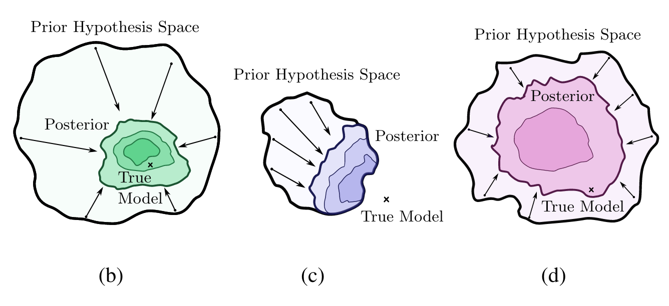
Within a Bayesian framework, we want the posterior $p(\mathcal{D}|\mathcal{M})$ to converge towards the correct solution while respecting the appropriate inductive bias. For this, the prior hypothesis space, also known as support, must be large enough to encompass the true model, as depicted in Figure 2. If the inductive bias aligns with the true model, and the true model lies within the prior hypothesis space (scenario (b) in the figure, akin to the CNN case), the model will contract around the accurate solution.

However, if the prior hypothesis space is too restricted, limiting the model's flexibility, it may not include the correct solution, even if the inductive bias is accurate. Consequently, the posterior will contract towards an incorrect solution, as illustrated by the example of the linear function.

Furthermore, when the support is excessively broad, and the model lacks the appropriate inductive bias, the model will not effectively contract (depicted in Figure 2(d), representing the MLP example). In such cases, the model's ability to converge to the correct solution is impaired.

In practical terms, our choice of a model involves finding a balance between flexibility and support. We aim to select a highly flexible model that can cover a wide range of possibilities (large support). However, to ensure sensible inductive biases, we need to complement this flexibility with a suitable choice of prior $p(\boldsymbol{\theta})$ on the coefficients that govern the distribution over functions $p(f(\boldsymbol{x}))$ .^[7]

Double Descent

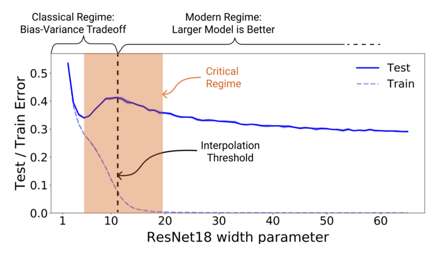
Traditional neural networks suffer from what is referred to as double descent, as depicted in Figure 3. In the classical regime, governed by the bias-variance tradeoff, as model complexity increases the expected test error initially decreases, reaches a minimum, and then starts increasing due to overfitting. However, double descent challenges this conventional understanding and introduces a new perspective. It reveals that, with sufficiently large datasets, there exists a second descent in the error curve, referred to as the modern interpolating regime, occurring after the initial peak of overfitting. This unexpected behavior suggests that complex models can still generalize well and achieve lower test errors, even after the conventional overfitting point.

Wilson et al.^[6] demonstrated that, with Bayesian model averaging over a suitable posterior approximation and sensible priors, the unexpected double descent behavior seen in traditional approaches does not manifest in Bayesian deep learning models. Instead, we recover the expected monotonic behavior, where accuracy improves as model flexibility increases. This will be further elaborated in the section on double descent revisited.

General optimization procedure

In a standard machine learning optimization process for a supervised problem, given a dataset $\mathcal{D}=\left\{\left(\boldsymbol{x}_n \in \mathbb{R}^N, \boldsymbol{y}_n \in \mathbb{R}^M\right)\right\}$ , where $\boldsymbol{y}_n \in \mathbb{R}^M$ for regression and $\boldsymbol{y}_n \in \{0,1\}^M$ for binary classification, we typically perform Maximum Likelihood Estimation. The objective is to find the optimal parameters $\boldsymbol{\theta} \in \mathbb{R}^P$ , which correspond to the weights and biases in a typical multi-layer perceptron, for example. This optimization process is formulated as follows:

\hat{\boldsymbol{\theta}}_{\text{MLE}} = \underset{\boldsymbol{\theta} \in \Theta}{\operatorname{argmax}}\; p(\mathcal{D} |\boldsymbol{\theta}).

The optimization strategy is frequently reformulated as a minimization problem.^[7] To further mitigate overfitting, a penalty term $C(\boldsymbol{\theta})$ (regularizer) is commonly incorporated. This modified minimization strategy is known as empirical risk minimization and can be expressed as follows:

\hat{\boldsymbol{\theta}}=\underset{\boldsymbol{\theta} \in \Theta}{\operatorname{argmin}}\; \left[ - \log p(\mathcal{D}|\boldsymbol{\theta}) + \lambda C(\boldsymbol{\theta}) \right],

where $\lambda \geq 0$ serves as a tunable regularization parameter.

In the frequentist framework, we consider $\boldsymbol{\theta}$ as a fixed but unknown parameter that solely depends on the data. In contrast, the Bayesian framework treats all unknowns as random variables. Consequently, we hold prior beliefs about the distribution $p(\boldsymbol{\theta})$ , and upon observing the data, we update these beliefs using the posterior distribution $p(\boldsymbol{\theta}|\boldsymbol{x})$ . The Maximum A Posteriori (MAP) framework aligns more closely with Bayesian principles, as it aims to maximize the posterior expression (1):

\hat{\boldsymbol{\theta}}_{\text{MAP}} = \underset{\boldsymbol{\theta} \in \Theta}{\operatorname{argmax}}\; p(\boldsymbol{\theta}|\mathcal{D}) \propto \underset{\boldsymbol{\theta} \in \Theta}{\operatorname{argmax}}\; p(\boldsymbol{\theta}) p(\mathcal{D}|\boldsymbol{\theta}).

If we consider i.i.d. samples, the likelihood factorizes into conditional probabilities:

p(\mathcal{D} | \boldsymbol{\theta}) = \prod_{n=1}^N p\left(\boldsymbol{y}_n | \boldsymbol{f}(\boldsymbol{x}_n, \boldsymbol{\theta})\right),

where we introduce the feature function $\boldsymbol{f}(\boldsymbol{\theta}, \boldsymbol{x})$ with $\boldsymbol{\theta}\in \mathbb{R}^P$ , which predicts the outputs of the output distribution (e.g., a Gaussian). Reformulating as a minimization problem using log-loss, we obtain the following optimization strategy:

\begin{aligned} \hat{\boldsymbol{\theta}}_{\text{MAP}} &=\underset{\boldsymbol{\theta} \in \Theta}{\operatorname{argmin}}\; \left( - \log p(\boldsymbol{\theta}) + \sum_{n = 1}^N \ell_n(\boldsymbol{x}_n, \boldsymbol{y}_n, \boldsymbol{\theta}) \right) \\ & = \underset{\boldsymbol{\theta} \in \Theta}{\operatorname{argmin}}\; \mathcal{L}(\boldsymbol{x}_n, \boldsymbol{y}_n, \boldsymbol{\theta}), \end{aligned}

where we define the empirical loss $\ell_n$ and log joint distribution $\mathcal{L}$ as follows:

\begin{aligned} \ell_n(\boldsymbol{x}_n, \boldsymbol{y}_n, \boldsymbol{\theta})&=-\log p\left(\boldsymbol{y}_n | \boldsymbol{f} (\boldsymbol{x}_n, \boldsymbol{\theta})\right), \\ \mathcal{L} (\boldsymbol{x}_n, \boldsymbol{y}_n, \boldsymbol{\theta}) &= - \left[\sum_{n=1}^{N} \log p\left(\boldsymbol{y}_{n} | \boldsymbol{f}\left(\boldsymbol{x}_{n}, \boldsymbol{\theta}\right)\right)+\log p(\boldsymbol{\theta}) \right]. \end{aligned}

Note that the regularized MLE estimate is recovered from the regularized empirical risk problem by setting the complexity parameter to $C(\boldsymbol{\theta}) = - \log p(\boldsymbol{\theta})$ with $\lambda = 1$ .

Posterior Approximations

Maximum A Posteriori estimation

The simplest approximate inference method involves computing the Maximum A Posteriori (MAP) estimate:

\hat{\boldsymbol{\theta}}=\operatorname{argmax} p(\boldsymbol{\theta} | \mathcal{D})=\operatorname{argmax} \log p(\boldsymbol{\theta})+\log p(\mathcal{D} | \boldsymbol{\theta}).

Here, we assume that the posterior concentrates all its probability mass on a single value:

p(\boldsymbol{\theta} | \mathcal{D}) \approx \delta(\boldsymbol{\theta}-\hat{\boldsymbol{\theta}}),

which corresponds to a typical machine learning approach where a single set of optimal parameters is chosen. However, such a procedure has several drawbacks, including a lack of uncertainty quantification for the parameters and limited utilization of Bayesian methods. In a Bayesian framework, we have the opportunity to use other model selection processes that have been shown to improve accuracy.

To capture the uncertainty effectively, we can employ various inference algorithms, including but not limited to the grid approximation, variational inference, Markov Chain Monte Carlo (MCMC), and the Laplace approximation. These methods allow for a better characterization of parameter uncertainty and enable the full potential of Bayesian approaches.

Laplace Approximation

To provide further insight, we reframe the posterior expression (1) as follows:

p(\boldsymbol{\theta} |\mathcal{D}) = \frac{p(\boldsymbol{\theta}) p(\mathcal{D} | \boldsymbol{\theta})}{p(\mathcal{D})} = \frac{p(\mathcal{D}, \boldsymbol{\theta})}{p(\mathcal{D})},

where, in the second step, we use the property that the conditional probability can be expressed as the quotient of the joint probability with respect to the marginal. Within the Laplace approximation,^[8] we assume that we can represent this posterior as a multivariate Gaussian:

p(\boldsymbol{\theta}|\mathcal{D}) =\frac{1}{Z} e^{- \mathcal{E}(\boldsymbol{\theta})} \quad \text{with} \quad \mathcal{E}(\boldsymbol{\theta}) = - \log p(\boldsymbol{\theta}, \mathcal{D}),

where $\mathcal{E}(\boldsymbol{\theta})$ (corresponding to the loss function in the MAP estimate) is referred to as the energy function. The normalization constant, $Z = p(\mathcal{D}) = \int p(\mathcal{D} | \boldsymbol{\theta}) p(\boldsymbol{\theta})\, d \theta$ , serves as an analogy to the canonical ensemble in statistical physics.

By performing a Taylor expansion of the posterior approximation around the lowest energy state $\hat{\boldsymbol{\theta}}$ (obtained, for example, using any standard machine learning optimization with regularized empirical risk minimization or the simple MAP approach explained above), we arrive at the following expression:

\begin{aligned} \mathcal{E}(\boldsymbol{\theta}) &\simeq \mathcal{E}(\hat{\boldsymbol{\theta}}_{\text{MAP}}) + (\boldsymbol{\theta} - \hat{\boldsymbol{\theta}}_{\text{MAP}})^T \boldsymbol{\nabla}_\theta \mathcal{E}(\boldsymbol{\theta}) \\ & + \frac{1}{2}(\boldsymbol{\theta} - \hat{\boldsymbol{\theta}}_{\text{MAP}})^T \left(\boldsymbol{\nabla}^2_\theta \mathcal{E}(\boldsymbol{\theta}) \mid_{\hat{\boldsymbol{\theta}}_{\text{MAP}}}\right) (\boldsymbol{\theta} - \hat{\boldsymbol{\theta}}_{\text{MAP}}). \end{aligned}

The first term vanishes at the mode $\hat{\boldsymbol{\theta}}_{\text{MAP}}$ since the gradient is zero. Consequently, we obtain the joint probability distribution:

\begin{aligned} \hat{p}(\mathcal{D}, \boldsymbol{\theta}) & \simeq e^{- \mathcal{E}(\hat{\boldsymbol{\theta}})} \\ & \times \exp\left[-\tfrac{1}{2}(\boldsymbol{\theta} - \hat{\boldsymbol{\theta}}_{\text{MAP}})^T \left(\boldsymbol{\nabla}^2_\theta \mathcal{E}(\boldsymbol{\theta}) \mid_{\hat{\boldsymbol{\theta}}_{\text{MAP}}}\right) (\boldsymbol{\theta} - \hat{\boldsymbol{\theta}}_{\text{MAP}})\right], \end{aligned}

which, by comparing (11) and (12), yields the following posterior approximation:

p(\boldsymbol{\theta}|\mathcal{D}) = \frac{1}{Z} \hat{p}(\boldsymbol{\theta}, \mathcal{D}) \simeq \mathcal{N}(\boldsymbol{\theta}\mid \hat{\boldsymbol{\theta}}_{\text{MAP}}, \boldsymbol{\Sigma}),

where

\boldsymbol{\Sigma} = \left( \boldsymbol{\nabla}^2_\theta \mathcal{E}(\boldsymbol{\theta}) \mid_{\hat{\boldsymbol{\theta}}_{\text{MAP}}}\right)^{-1},

and $\boldsymbol{\Sigma}$ is the inverse of the Hessian.

The normalizing constant $Z$ corresponding to the marginal likelihood or evidence can be determined by the general formulation of a multivariate Gaussian and is given by

Z \simeq e^{- \mathcal{E}(\hat{\boldsymbol{\theta}})} (2\pi)^{D/2} (\det \boldsymbol{\Sigma})^{1/2}.

To explicitly compute the Hessian, we need to evaluate it for the joint log expression $\mathcal{L}$ from equation (8). For now, we will neglect the prior term $p(\boldsymbol{\theta})$ and focus on the log-likelihood term for each data point. The first and second derivatives are as follows:

\begin{aligned} \boldsymbol{\nabla}_{\boldsymbol{\theta}} \log p(\boldsymbol{y} \mid \boldsymbol{f}(\boldsymbol{x}, \boldsymbol{\theta})) & =\mathbf{J}_{\boldsymbol{\theta}}(\boldsymbol{x})^{\top} \boldsymbol{r}(\boldsymbol{y} ; \boldsymbol{f}), \\ \boldsymbol{\nabla}_{\boldsymbol{\theta}}^2 \log p(\boldsymbol{y} \mid \boldsymbol{f}(\boldsymbol{x}, \boldsymbol{\theta})) & =\mathbf{H}_{\boldsymbol{\theta}}(\boldsymbol{x})^{\top} \boldsymbol{r}(\boldsymbol{y} ; \boldsymbol{f}) \\ &-\mathbf{J}_{\boldsymbol{\theta}}(\boldsymbol{x})^{\top} \boldsymbol{\Lambda}(\boldsymbol{y} ; \boldsymbol{f}) \mathbf{J}_{\boldsymbol{\theta}}(\boldsymbol{\theta}), \end{aligned}

where $\mathbf{J}_{\boldsymbol{\theta}}(\boldsymbol{x})_{ci} = \partial f_c(\boldsymbol{\theta}, \boldsymbol{x})/\partial \theta_i \in \mathbb{R}^{M \times P}$ is the Jacobian (recall $M$ is the dimension of the output and $P$ the dimension of the parameters $\boldsymbol{\theta}$ ), $\left[\mathbf{H}_{\boldsymbol{\theta}}(\mathbf{x})\right]_{c i j}=\frac{\partial^{2} f_{c}(\mathbf{x}, \boldsymbol{\theta})}{\partial \theta_{i} \partial \theta_{j}} \in \mathbb{R}^{C \times M \times M}$ the Hessian tensor, $\mathbf{r}(\boldsymbol{y}; \boldsymbol{f}) = \boldsymbol{\nabla}_{\boldsymbol{f}} \log p(\boldsymbol{y} | \boldsymbol{f})$ the residual, and $\boldsymbol{\Lambda}(\boldsymbol{y} ; \boldsymbol{f})=-\boldsymbol{\nabla}_{\boldsymbol{f f}}^{2} \log p(\boldsymbol{y} | \boldsymbol{f})$ the per-input noise term.

In general, when considering the prior, we have the flexibility to choose any twice-differentiable log-density prior $p(\boldsymbol{\theta})$ . However, even for a simple case like the weight-decay regularizer $C(\boldsymbol{\theta}) = \frac{1}{2} \gamma^{-2} |\theta|^2$ , where we assume a zero-mean Gaussian prior $\mathcal{N}(\theta|0, \gamma^2 I)$ , scalability issues arise. For a supervised learning setting, the Hessian at the MAP estimate is given by:

\boldsymbol{\nabla}^2_{\boldsymbol{\theta}} \mathcal{E}(\boldsymbol{\theta}) \mid_{\hat{\boldsymbol{\theta}}_{\text{MAP}}} = -\gamma^{-2} I - \sum_{n = 1}^N \boldsymbol{\nabla}_{\boldsymbol{\theta}}^2 \log p(y_n | \boldsymbol{f}(x_n, \boldsymbol{\theta})) \mid_{\hat{\boldsymbol{\theta}}_{\text{MAP}}}.

The second term in this equation scales quadratically with the number of network parameters, making it computationally infeasible for large networks with millions of parameters. Additionally, for most neural networks, the log-likelihood is not convex, leading to a non-positive-definite Hessian. Consequently, we encounter two significant challenges: (1) the optimization problem is non-convex, making it difficult to find a suitable global minimum, and (2) the optimization procedure becomes more unstable in general.

Gauss-Newton approximation

One way to address the scalability issues is to perform a Gauss-Newton approximation to the Hessian. This involves neglecting the Hessian-tensor term in (18), effectively linearizing the equation:

\boldsymbol{\nabla}_{\boldsymbol{\theta}}^2 \log p(\boldsymbol{y} \mid \boldsymbol{f}(\boldsymbol{x}, \boldsymbol{\theta})) \simeq \mathbf{J}_{\boldsymbol{\theta}}(\boldsymbol{x})^{\top} \boldsymbol{\Lambda}(\boldsymbol{y} ; \boldsymbol{f}) \mathbf{J}_{\boldsymbol{\theta}}(\boldsymbol{x}),

where $\mathbf{J}_{\boldsymbol{\theta}}(\boldsymbol{x})$ is the Jacobian matrix and $\boldsymbol{\Lambda}(\boldsymbol{y} ; \boldsymbol{f})$ is a diagonal matrix containing the second derivatives of the log-likelihood with respect to the output predictions. This approximation also ensures that the optimization remains positive semi-definite. Additionally, computing Jacobians involves only first-order derivatives, which are efficiently implemented in many modern machine learning tools.

For the common choice of a Gaussian prior $p(\boldsymbol{\theta}) = \mathcal{N}(\boldsymbol{\theta} | \boldsymbol{\mu}, \boldsymbol{\beta})$ , the Laplace approximation simplifies to:

p(\boldsymbol{\theta} | \mathcal{D}) \approx \mathcal{N}(\boldsymbol{\theta}, \boldsymbol{\Sigma}_{\mathrm{GGN}}),

where

\boldsymbol{\Sigma}_{\mathrm{GGN}}^{-1}=\sum_{n=1}^{N} \mathbf{J}_{\boldsymbol{\theta}}\left(\boldsymbol{x}_{n}\right)^{\top} \boldsymbol{\Lambda}\left(\boldsymbol{y}_{n} , \boldsymbol{f}_{n}\right) \mathbf{J}_{\boldsymbol{\theta}}\left(\boldsymbol{x}_{n}\right)+\boldsymbol{\beta}^{-1}.

However, inverting this matrix still takes $\mathcal{O}(P^3)$ . Therefore, additional approximation schemes are necessary for such cases. One simple approach is diagonal factorization, which ignores off-diagonal terms in the matrix.

In summary, the Laplace approximation is favored for its simplicity as an inference approximation scheme. Apart from computing the MAP estimate, which can be accomplished using traditional optimization algorithms, the main computational requirement is to calculate the inverse of the Hessian matrix at $\boldsymbol{\theta}_{\text{MAP}}$ . This straightforward implementation makes it suitable for obtaining statistical measures of pre-trained models and has been conveniently implemented in PyTorch by Immer et al.^[9] in the Laplace Redux library. Moreover, the Laplace approximation provides a reasonable approximation for models with moderate parameter dimensions.

Challenges arise, however, once the Laplace approximation is applied to deep models with very many parameters. The high dimensionality makes inverting the Hessian expensive, and for very large neural networks the approach may become impractical. In that regime, sampling methods like Markov Chain Monte Carlo or variational inference are often preferred for estimating parameter uncertainty.

Variational Inference

Methods like Monte Carlo Markov Chain algorithms have proven to be effective for sampling from exact posteriors. However, they also encounter scalability issues, primarily because they may require a large number of iterations until the algorithm converges to the stationary distribution (i.e., the desired posterior). This slow convergence can make MCMC computationally expensive and impractical for large-scale problems.

Alternatively, a popular method is Variational Inference, also known as variational Bayes. In this approach, we propose an approximate distribution (referred to as the variational distribution) that belongs to a tractable family of distributions $\mathcal{Q}$ parameterized by a set of parameters $\boldsymbol{\phi}$ . The goal is to find the best approximate solution to the intractable posterior $p(\boldsymbol{\theta}|\mathcal{D})$ :

q^*=\underset{q \in \mathcal{Q}}{\operatorname{argmin}}\; D(q \,\|\, p),

where $D(q \,\|\, p)$ is typically the Kullback-Leibler divergence between the exact posterior and the variational distribution, defined as:

D_{\text{KL}}(q \,\|\, p) = \int_{\boldsymbol{\theta}'} q(\boldsymbol{\theta}'|\boldsymbol{\phi}) \log \left( \frac{q(\boldsymbol{\theta}'|\boldsymbol{\phi})}{p(\boldsymbol{\theta}'|\mathcal{D})} \right) d\boldsymbol{\theta}'.

The above expression quantifies the discrepancy between the approximate and exact posterior distributions. Instead of directly minimizing the divergence, a more convenient quantity, known as the Evidence Lower Bound (ELBO), can be used, which is related to the KL divergence. The ELBO is defined as:

\mathbb{E}_{q(\boldsymbol{\theta} | \boldsymbol{\phi})}\left[\log p(\mathcal{D} | \boldsymbol{\theta})+\log p(\boldsymbol{\theta})-\log q(\boldsymbol{\theta} | \boldsymbol{\phi})\right].

By maximizing the ELBO, we effectively minimize the KL divergence, thereby making the variational distribution closer to the true posterior. Since the ELBO involves an expectation with respect to the variational distribution, it still requires some calculation of the often intractable posterior $p(\boldsymbol{\theta}|\mathcal{D})$ .

The most common choice for the posterior approximation is to use multivariate Gaussians, which take the form $q(\boldsymbol{\theta}|\boldsymbol{\phi}) = \mathcal{N}(\boldsymbol{\theta}|\boldsymbol{\mu}, \boldsymbol{\Sigma})$ . In this case, the parameters $\boldsymbol{\phi}$ consist of the mean $\boldsymbol{\mu}$ and the covariance matrix $\boldsymbol{\Sigma}$ of the Gaussian distribution. This approach differs from the Laplace approximation, where the posterior covariance was derived from the Hessian at the MAP estimate (as shown in equations (15) and (16)).

The variational approximation offers a more global representation of the posterior, but it still faces challenges: it can settle in suboptimal minima and is limited to a specific class of functions $q \in \mathcal{Q}$ , much like the Laplace approximation. Notably, the use of Gaussian distributions for the approximate posterior might restrict its expressiveness, unlike methods like MCMC, which do not impose such assumptions and can explore more diverse posteriors.^[10]

Deep Ensembles

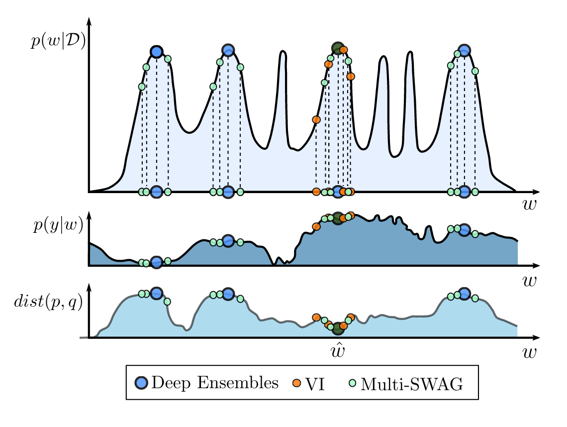
To address this, other approaches like Deep Ensembles have been proposed, which involve training multiple models with different initialization to capture the uncertainty and explore different regions of the parameter space. These ensembles can provide a more robust and comprehensive representation of the often multi-modal posterior distribution, as illustrated in Figure 4. In this ensemble-based approach, the models are equally weighted by a sum of Dirac delta functions, with each function allocating mass to the MAP mode of a specific model $m$ :

p(\boldsymbol{\theta} | \mathcal{D}) \approx \frac{1}{M} \sum_{m=1}^M \delta\left(\boldsymbol{\theta}-\hat{\boldsymbol{\theta}}_{\text{MAP}}^m\right).

Here, $M$ represents the number of models in the ensemble, and $\hat{\boldsymbol{\theta}}_{\text{MAP}}^m$ denotes the MAP estimate for model $m$ .

Multi-SWAG

Multi-SWAG^[6] builds upon the Deep Ensemble concept and adds an extra layer of complexity by fitting a Gaussian to each of the local modes, often referred to as basins of attraction, represented by the MAP estimates $\hat{\boldsymbol{\theta}}_{\text{MAP}}^m$ . This is achieved using the SWAG (Stochastic Weight Averaging Gaussian) approximation, which provides a method to fit these Gaussians (though we will not delve into its details here). As a result, the posterior distribution is approximated as a mixture of Gaussian components:

p(\boldsymbol{\theta} | \mathcal{D}) \approx \frac{1}{M} \sum_{m=1}^M \mathcal{N}\left(\boldsymbol{\theta} | \hat{\boldsymbol{\theta}}_m, \boldsymbol{\Sigma}_m\right).

The key advantage over simple Deep Ensembles lies in the ability to directly generate new posterior samples at each mode, thanks to the mixture-of-Gaussians representation. This approach provides a more fine-grained approximation of the posterior distribution, allowing for better exploration of the parameter space and a more comprehensive understanding of model uncertainty.

Comparison of posterior approximations

To compare the computation of the predictive distribution using different methods, namely deep ensembles, variational inference for a single basin, and Multi-SWAG, Wilson et al.^[6] employed an illustrative example depicted in Figure 4. Recall that the posterior predictive distribution is the integral of the conditional predictive and the posterior, both of which are shown in the top and middle plots respectively. As such, we want the product of the two to be as large as possible.

Variational inference selects samples from a single basin of attraction in the posterior $p(\boldsymbol{\theta}|\mathcal{D})$ , corresponding to parameters $\boldsymbol{\theta}$ where the Kullback-Leibler divergence between the true posterior and the approximate posterior is minimized, as depicted in the bottom plot. On the other hand, Deep Ensembles considers multiple basins of attraction due to being an ensemble of models with different setups, each potentially having a different MAP estimate $\hat{\boldsymbol{\theta}}_{\text{MAP}}^m$ . Understanding how the conditional predictive distribution $p(\boldsymbol{y}| \boldsymbol{x}, \boldsymbol{\theta})$ varies with respect to the parameters (as seen in the middle plot) reveals the benefits of sampling from different basins.

Although the probability mass for basins of attraction other than the one chosen by variational inference might be lower, their large posterior predictions can still have a substantial impact on the overall posterior predictive distribution. Consequently, when samples are obtained near $\hat{\boldsymbol{\theta}}$ ( $\hat{\omega}$ in the plot), Deep Ensembles and Multi-SWAG show significant improvements in the posterior predictive compared to variational inference by sampling from additional modes in different basins.

To summarize: having multiple basins of attraction, obtained by distinct components of the ensemble, leads to greater functional diversity compared to Bayesian approaches that primarily concentrate on approximating the posterior within a single basin of attraction.

Back to Double Descent

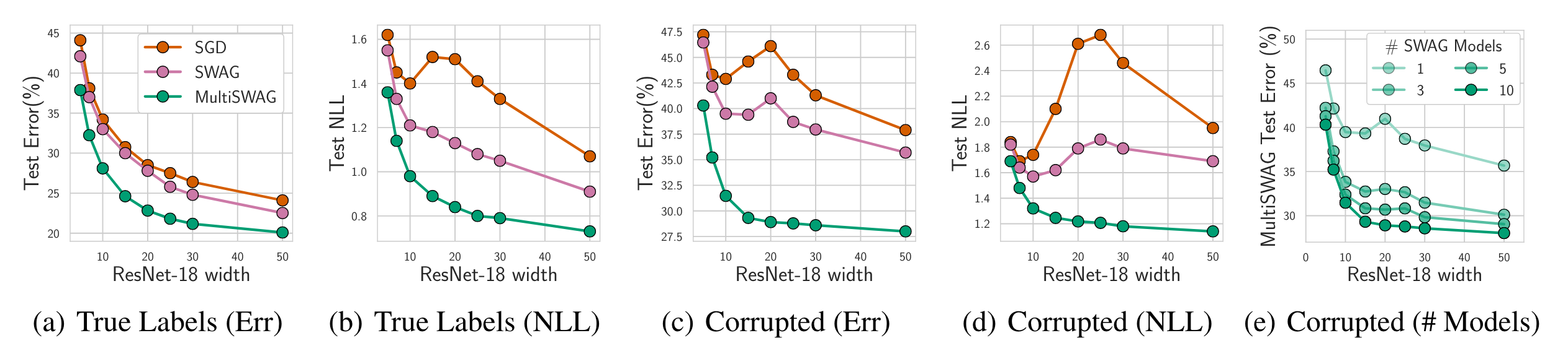
With the insights gained from the previous section, we can now understand the claim made by Wilson et al.^[6] that Bayesian neural networks do not exhibit double descent behavior. This boils down to their ability (for certain approximations as we will see) to perform an exhaustive multimodal Bayesian model average. To examine this hypothesis further, they conducted experiments using Multi-SWAG, SWAG, and SGD with ResNet-18 models of varying widths. The results for error and negative log-likelihood (NLL) are illustrated in Figure 5. These experiments were also conducted on a partially corrupted dataset, where 20% of the labels were randomly reshuffled (Figures 5(c) and 5(d)).

The error plot 5(a) clearly shows the traditional double descent behavior for SWAG. However, Multi-SWAG effectively mitigates the issue of double descent by implementing a comprehensive multimodal Bayesian model averaging approach. As a result, the error curve scales monotonically with increasing model flexibility, demonstrating the model's ability to adapt to different complexities while avoiding the double descent phenomenon.

Test error and NLL versus ResNet-18 width for SGD, SWAG and Multi-SWAG — Figure 5. Figure taken from [6]. Plot (a) the test error and (b) test negative log-likelihood for the uncorrupted dataset with respect to the ResNet-18 width. In (c) and (d) we find the test error and NLL for a partially corrupted dataset. In plot (e) we find the test error for Multi-SWAG with a varying number of SWAG models for the corrupted dataset. We observe that with an increasing number of SWAG models we reduce the double descent behaviour monotonically.

Application of BNNs in Cosmology

In this section, we summarize the main results of Lemos et al.,^[11] in which a BNN framework is studied for simulation-based inference (SBI) methods in cosmology. The generalization and the reliability of an SBI outside the training set are highly dependent on the goodness of the simulations and the large computational expense of generating all possible parameter combinations. A particularly relevant SBI method in cosmology is Density Estimation Likelihood-Free Inference (DELFI),^[12] which makes use of simulations to estimate the likelihood of the model and allows one to perform Bayesian inference free from any likelihood assumptions.

In some cases, it is challenging to evaluate the likelihood function explicitly due to the complexity of the model or the high dimensionality of the data. In likelihood-free inference methods like DELFI, the goal is to perform Bayesian parameter inference without explicitly computing the likelihood function. Instead, it focuses on estimating the posterior distribution directly from the data.

The key steps involved in DELFI are as follows:

Simulator: A simulator is used to generate synthetic data based on the given model and parameter values drawn from priors. These simulations represent the model's predictions for various parameter settings.
Summary Statistics: Summary statistics are calculated from both the synthetic data and the observed data. Data compression schemes should be carefully designed to reduce the data to the smallest set possible, whilst retaining as much information about the parameters of interest as possible.
Density Estimation: Using summary statistics, density estimation methods, such as neural networks, are employed to approximate the likelihood function. These methods learn the mapping between the summary statistics and the parameters.
Posterior Inference: Once the density estimation has been performed, the posterior distribution of the parameters can be estimated using MCMC or other sampling or variational techniques.

Simulator

For the scope of the SBI, simulations of the CMB power spectrum are chosen, because they are computationally cheap to generate and it is possible to write down a likelihood to perform a likelihood-based analysis.

CAMB^[13] generates a suite of 100,000 CMB power spectra with $l_{\max}=2500$ , and only the power spectrum of temperature anisotropies is used.
The Planck 2018 TT^[14] native likelihood is used in the code cobaya,^[15] to convert this power spectrum into a binned power spectrum, at 215 multipole bins.
Planck TT data and covariance matrix are used in the same likelihood as the observed data and error model, respectively.

The simulations are drawn from the uniform priors shown in the table below.

Parameter	Prior
$H_0$	$\mathcal{U}(50,90)$
$\Omega_b h^2$	$\mathcal{U}(0.01,0.05)$
$\Omega_c h^2$	$\mathcal{U}(0.01,0.5)$
$\log(10^{10} A_s)$	$\mathcal{U}(1.5,3.5)$
$n_s$	$\mathcal{U}(0.8,1)$

Analysis

DELFI with data compression

A neural compressor, which is a neural network with 6 hidden layers of 128 neurons each, compresses the data to the dimensionality of the parameter space. The prediction of this neural network is used as the compressed data in the DELFI analysis.^[12] Then a masked autoregressive flow (MAF) is used as a density estimator.

DELFI without data compression

It is possible to perform density estimation directly on the data without the need for a compression algorithm. Mixture Density Networks (MDN) are used for density estimation, instead of MAFs.

DELFI without data compression and with weight marginalization

Next, the DELFI analysis is repeated with MDN, but applying Stochastic Weight Averaging (SWA) to perform marginalization over neural network parameters. This method provides an estimate of the weight uncertainty, and therefore the uncertainty on the predictions.

DELFI with data compression and with weight marginalization

Finally, the DELFI analysis is repeated with explicit massive compression through a regression network, adding marginalization to the neural network weights. MDN is then applied to the compressed data. Weight marginalization is used on both the compression and the MDN.

Results and Conclusions

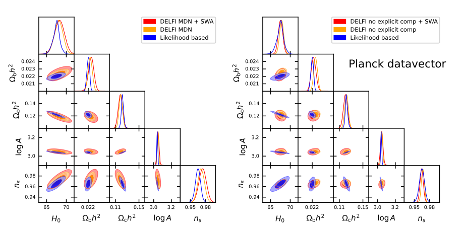
Marginalized posterior distributions for the DELFI variants — Figure 6. Figure extracted from [11]. Marginalized posterior distributions for the different variations of DELFI are presented. The left plot shows the results for DELFI without explicit compression, using an MDN, with weight-marginalized results in red, and non-weight-marginalized in orange. In blue the likelihood-based analysis is shown. The right plot shows the same for DELFI with compression through a regression network. The contours represent the 68% and 95% confidence intervals.

The results of applying all four versions of the DELFI analysis are shown in Figure 6. On the left panel, no explicit compression has been used. It is possible to see that the DELFI posteriors do correctly capture the degeneracies of the likelihood, as the ellipses are "tilted" in the same way as the real ones.

The size of both DELFI posteriors is larger than the likelihood-based one. This is due to the added epistemic uncertainty of having to estimate a likelihood from simulations.

When data compression is used with a neural compressor, it is not possible to fully recover the degeneracy directions.

Noise is introduced when running CAMB at the fiducial cosmology, and extra Gaussian noise is added at small scales $l>2000$ to test how the system behaves in the presence of unknown systematics or observational effects in the data that are not present in the simulation. Given that this extra noise has not been added to any of the training simulations, the observed data is different from any of the simulations the DELFI algorithm has been trained on.

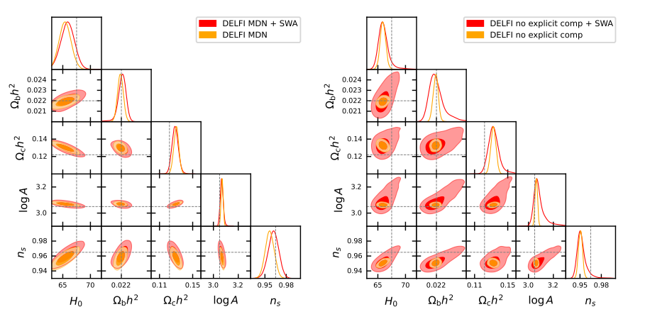
Marginalized posteriors using a synthetic data vector with added noise — Figure 7. Figure extracted from [11]. The same as Figure 6 using a synthetic data vector with added noise.

The results of the analysis are shown in Figure 7. Using no explicit compression, consistent results are obtained, but when there is no marginalization over the weights, some parameters show biased posteriors.

This shows that neural compression can lead to dangerous biases when the observed data is different from the simulations.

Marginalization of the neural network parameters thus prevents overfitting and increases the reliability of the posteriors, at the expense of slightly less confident posteriors.

References

K. Bykov, M. M.-C. Höhne, A. Creosteanu, K.-R. Müller, F. Klauschen, S. Nakajima, M. Kloft. Explaining Bayesian Neural Networks. arXiv:2108.10346 (2021).
S. Winter, T. Campbell, L. Lin, S. Srivastava, D. B. Dunson. Machine Learning and the Future of Bayesian Computation. arXiv:2304.11251 (2023).
S. Kullback, R. A. Leibler. On Information and Sufficiency. Ann. Math. Statist. 22(1), 79–86 (1951). doi:10.1214/aoms/1177729694.
C. Zhang, S. Bengio, M. Hardt, B. Recht, O. Vinyals. Understanding deep learning requires rethinking generalization. arXiv:1611.03530 (2017).
P. Nakkiran, G. Kaplun, Y. Bansal, T. Yang, B. Barak, I. Sutskever. Deep Double Descent: Where Bigger Models and More Data Hurt. arXiv:1912.02292 (2019).
A. G. Wilson, P. Izmailov. Bayesian Deep Learning and a Probabilistic Perspective of Generalization. arXiv:2002.08791 (2022).
K. P. Murphy. Probabilistic Machine Learning: An Introduction. MIT Press (2022).
E. Daxberger, A. Kristiadi, A. Immer, R. Eschenhagen, M. Bauer, P. Hennig. Laplace Redux: Effortless Bayesian Deep Learning. arXiv:2106.14806 (2022).
A. Immer, M. Korzepa, M. Bauer. Improving predictions of Bayesian neural nets via local linearization. AISTATS (2021).
L. V. Jospin, W. Buntine, F. Boussaid, H. Laga, M. Bennamoun. Hands-on Bayesian Neural Networks: A Tutorial for Deep Learning Users. IEEE Comput. Intell. Mag. 17(2), 29–48 (2022). arXiv:2007.06823.
P. Lemos, M. Cranmer, M. Abidi, C. Hahn, M. Eickenberg, E. Massara, D. Yallup, S. Ho. Robust Simulation-Based Inference in Cosmology with Bayesian Neural Networks. Mach. Learn.: Sci. Technol. 4, 01LT01 (2023). arXiv:2207.08435.
J. Alsing, B. Wandelt, S. Feeney. Massive optimal data compression and density estimation for scalable, likelihood-free inference in cosmology. MNRAS 477(3), 2874–2885 (2018). doi:10.1093/mnras/sty819.
A. Lewis, A. Challinor, A. Lasenby. Efficient Computation of Cosmic Microwave Background Anisotropies in Closed Friedmann–Robertson–Walker Models. ApJ 538, 473–476 (2000). doi:10.1086/309179.
Planck Collaboration. Planck 2018 results. VI. Cosmological parameters. A&A 641, A6 (2020). doi:10.1051/0004-6361/201833910.
J. Torrado, A. Lewis. Cobaya: code for Bayesian analysis of hierarchical physical models. JCAP 2021(05), 057. doi:10.1088/1475-7516/2021/05/057.